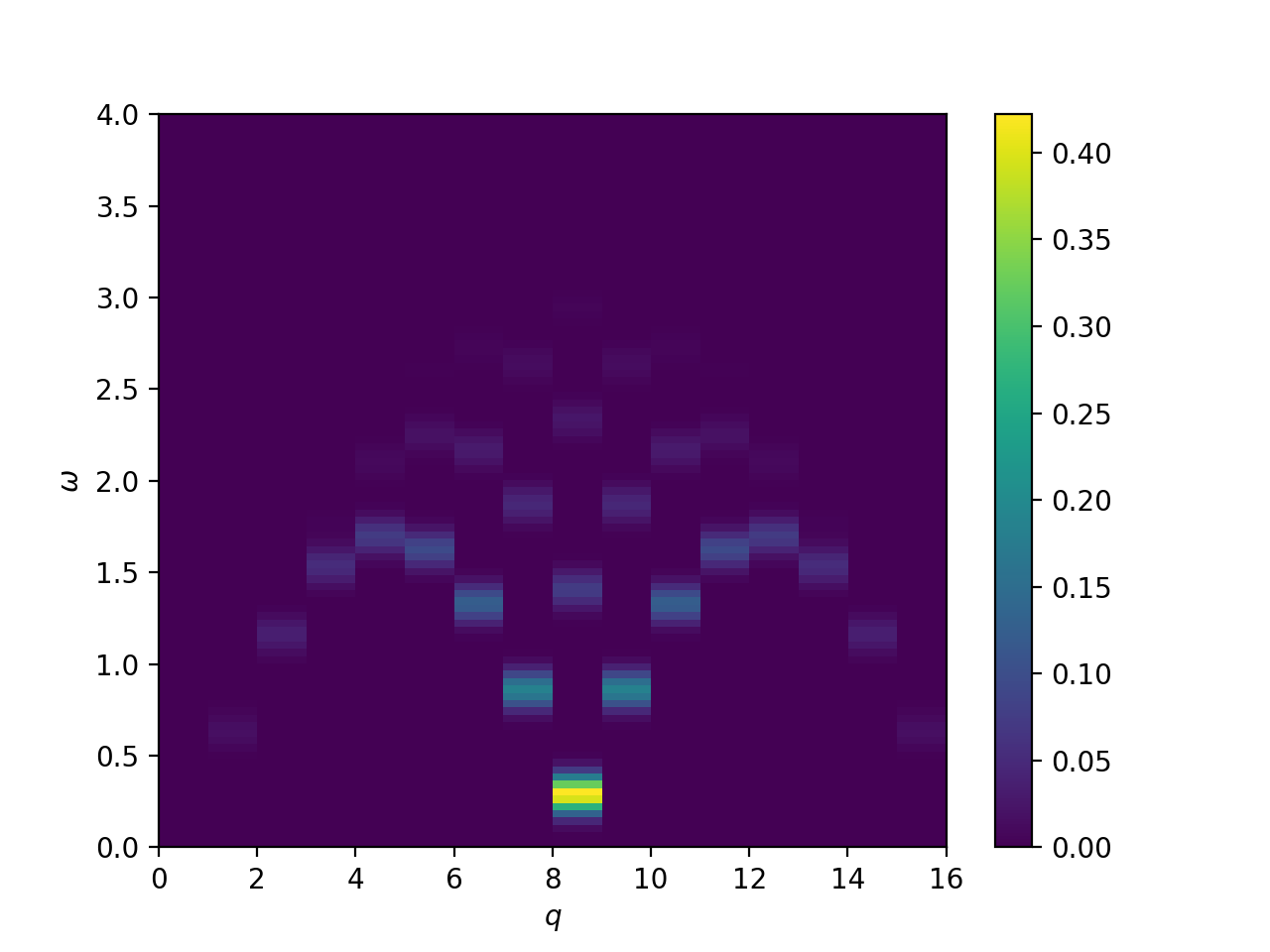
Dynamical structure factor of the Heisenberg S=1/2 chain, with momentum conservation

Dynamical structure factor of the Heisenberg S=1/2 chain

We compute the ground state energy of the \(S=1/2\) Heisenberg chain with periodic boundary conditions in each momentum sector \(k\). The Hamiltonian is given by

\[H = J\sum_{\langle i,j \rangle} \mathbf{S}_i \cdot \mathbf{S}_j\]

where \(\mathbf{S}_i = (S_i^x, S_i^y, S_i^z)\) are the spin \(S=1/2\) operators and \(\langle i,j \rangle\) denotes summation over nearest-meighbor sites \(i\) and \(j\). We set \(J=1\).

First, the Lanczos coefficients are computed using hydra and written to file

#include <hydra/all.h>

int main() {
  using namespace hydra;
  using namespace arma;

  int n_sites = 16;
  int n_up = n_sites / 2;

  // Create nearest-neighbor Heisenberg model
  BondList bonds;
  for (int s = 0; s < n_sites; ++s) {
    bonds << Bond("HB", "J", {s, (s + 1) % n_sites});
  }
  bonds["J"] = 1.0;

  // compute groundstate (known to be at k=0)
  Log("Computing ground state ...");
  auto block = Spinhalf(n_sites, n_up);
  auto gs = groundstate(bonds, block);
  Log("done.");

  for (int q = 0; q < n_sites; ++q) {

    Log("Dynamical Lanczos iterations for q={}", q);

    complex phase = exp(2i * pi * q / n_sites);
    BondList S_of_q;
    for (int s = 0; s < n_sites; ++s) {
      S_of_q << Bond("SZ", pow(phase, s) / n_sites, s);
    }

    // Compute S(q) |g.s.>
    auto v0 = zero_state(block);
    apply(S_of_q, gs, v0);
    double nrm = norm(v0);
    v0 /= nrm;

    // Perform 200 Lanczos iterations for dynamics starting from v0
    auto tmat = lanczos_eigenvalues_inplace(bonds, block, v0.vector(), 0, 0.,
                                            200, 1e-7);
    auto alphas = tmat.alphas();
    auto betas = tmat.betas();

    // Write alphas, betas, and norm to file for further processing
    alphas.save(
        fmt::format("outfiles/alphas.N.{}.nup.{}.q.{}.txt", n_sites, n_up, q),
        raw_ascii);
    betas.save(
        fmt::format("outfiles/alphas.N.{}.nup.{}.q.{}.txt", n_sites, n_up, q),
        raw_ascii);
    std::ofstream of;
    of.open(
        fmt::format("outfiles/norm.N.{}.nup.{}.q.{}.txt", n_sites, n_up, q));
    of << nrm;
    of.close();
  }

  return EXIT_SUCCESS;
}

The produced data is the read from file and can be visualized using the following python script.

#!/usr/bin/env python
import numpy as np
import matplotlib.pyplot as plt

n_sites = 16
n_up = n_sites // 2

eta = 0.05
n_omegas = 100
max_omega = 4.0
omegas = np.linspace(0, max_omega, n_omegas)

# compute broadened spectrum
spectra = np.zeros((n_sites, n_omegas))
for q in range(n_sites):
    alphas = np.loadtxt("outfiles/alphas.N.{}.nup.{}.q.{}.txt".format(n_sites, n_up, q))
    betas = np.loadtxt("outfiles/betas.N.{}.nup.{}.q.{}.txt".format(n_sites, n_up, q))
    norm = np.loadtxt("outfiles/norm.N.{}.nup.{}.q.{}.txt".format(n_sites, n_up, q))

    # compute poles and weights from tridiagonal matrix
    tmat = np.diag(alphas[:50]) + np.diag(betas[:49], k=1) + np.diag(betas[:49], k=-1)
    eigs, evecs = np.linalg.eigh(tmat)
    e0 = eigs[0]
    poles = eigs - e0
    weights = (norm**2) * (evecs[0, :]**2)
    print(norm, e0)
    
    # compute broadened spectrum with Gaussian broadening eta
    diffs = np.subtract.outer(omegas, poles)
    gaussians = np.exp(-(diffs / (2*eta))**2) / (eta * np.sqrt(2*np.pi))
    spectra[q, :] = gaussians @ weights

p = plt.imshow(spectra.T, origin='lower', extent=[0, n_sites, 0, max_omega],
           interpolation=None, aspect='auto')
plt.xlabel(r"$q$")
plt.ylabel(r"$\omega$")
plt.colorbar(p)
plt.show()

This will plot the following image: