User guide

A step-by-step guide to using Hydra

Table of contents

1. Setting up your application
   1. Writing your code using hydra
   2. Compiling your code using hydra
2. Basics
   1. Hilbertspaces and operators
   2. Linear Algebra
   3. Hilbertspaces and blocks
   4. Operators
   5. Linear Algebra

Setting up your application

Writing your code using hydra

After having compiled the hydra library, it is time to write our first program in hydra. As hydra is a C++ library we will need to define a main routine, include the hydra headers, and load the hydra and arma namespaces.

#include <hydra/all.h>

int main() {
  using namespace hydra;
  using namespace arma;

  // Actual code goes here ....
  
  return EXIT_SUCCESS;
}

arma is the namespace for the linear algebra library Armadillo, which hydra is based on. These tasks have to performed for every code using hydra, so the above lines of code serve as a canvas for doing quantum many-body physics using hydra.

Compiling your code using hydra

Once you have written your code, say in a file called main.cpp, you will have to compile it in order to execute it. This requires you to tell the compiler the directory of the hydra header file <hydra/all.h>, and to link to the hydra library. Moreover, you will need to link your application to the Lapack/BLAS libraries. The easiest way to do all of this is to create a Makefile. On Linux systems this can be achieved by:

hydradir = /path/to/hydra
all:
	g++ main.cpp -o main -O2 -std=c++17 -I$(hydradir) -L$(hydradir)/lib -lhydra -llapack -lblas

On MacOS, the standard Lapack/BLAS routines for linear algebra are provided through the Accelerate framework. Thus, you could use the following Makefile:

hydradir = /path/to/hydra
all:
	g++ main.cpp -o main -O2 -std=c++17 -I$(hydradir) -L$(hydradir)/lib -lhydra -framework Accelerate

Once the Makefile is written you can simply call

make

to compile the code, and

./main

to run it. Alternatively, you might also decide on linking to the Intel MKL, see Compiling hydra using Intel MKL.

Basics

Hilbertspaces and operators

The fundamental objects in quantum mechancs are Hilbert spaces, operators and wave functions. These are alse central objects in Hydra. There are several Hilbert spaces defined in Hydra, like the [Spinhalf] To get started we want to create a simple exchange operator on two sites in a spin \(S=1/2\) Hilbert space.

First we create the Hilbertspace spanned by

This is done by constructing a Spinhalf object on two sites

auto block = Spinhalf(2);

The keyword c++ auto was introduced in C++11 and tells the compiler to automatically derive the type of an object. Next, we define the the exchange operator by creating a Bond object,

auto op = Bond("HB", {0, 1});

The first argument defines the type of the bond. Several special types are predefined. Alternatively, also a coupling matrix can be given as an argument instead of the string. The second argument is the array containing the number of sites the operator acts on, in this case 0 and 1. Hydra always starts counting at 0. For more details how to define local operators see …

Finally, we create the matrix of this operator in the computational basis and print it,

auto mat = matrix_real(op, block);
HydraPrint(mat);

Linear Algebra

We are not just interested in writing down matrices but in doing computations with them. Hence, we will need to perform basic linear algebra algorithms and routines on our constructed objects. To do so, hydra relies on the Armadillo library, which is a powerful and convenient linear algebra library for C++, which wraps the efficient Lapack and Blas routines.

We might, for example be interested in the eigenvalues of a matrix. In the above case, we know that the eigenvalues \(\varepsilon\) and eigenvectors of \(\vec{S}_i \cdot \vec{S}_j\) are simply,

for the singlet state, and

for the three triplet states. To compute this

Hilbertspaces and blocks

A physical system is typically described by a Hamiltonian operator acting on a Hilbert space. In this introductory material we will consider a simple example, the spin-\(1/2\) Heisenberg model on a periodic chain lattice. It’s Hilbert space \(\mathcal{H}\) is the tensor product of local spins \(\sigma_i = \uparrow,\downarrow\) on a lattice,

whose dimension grows exponentially with the number of lattice sites \(N\), \(\text{dim}(\mathcal{H}) = 2^N\). The Hamiltonian is given by,

Here, \(\vec{S}_i = (S^x_i, S^y_i, S^z_i)\) denotes the spin operators on site \(i\), and the sum \(\langle i,j \rangle\) denotes the sum over nearest-neighbors \(i,j\) on the lattice. Upon choosing a basis \(\vert n \rangle\) of \(\mathcal{H}\) we can compute the matrix elements of \(H_{mn} = \langle m \vert H \vert n \rangle\). In Hydra, we typically work in a basis of product states,

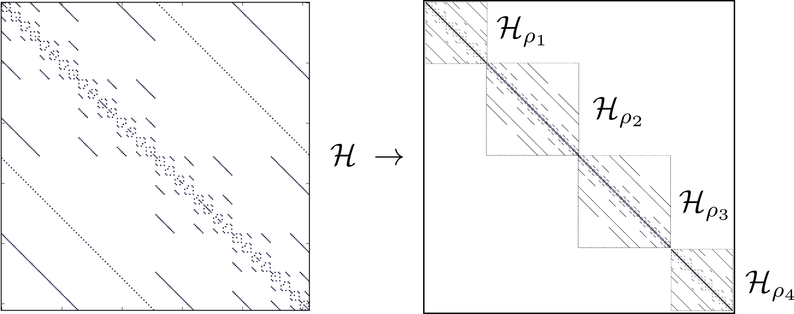
Representing the Hamiltonian \(H\) in this basis will yield a sparse matrix, whose non-zero matrix elements are distributed something like this:

Symmetries of \(H\) are operators \(S\), which commute with the Hamiltonian \([H,S] = 0\). We can choose a basis of the Hilbert space such that every state transforms according to an irreducible representation \(\rho\), also called quantum numbers, of the group of symmetries. If we express the Hamiltonian in this basis, it will attain a block diagonal form,

For the Heisenberg chain above, the symmetries include the continuous \(U(1)\) spin rotation symmetry,

The irreducible representations \(\rho\) are labeled by \(S^z_{\text{tot}} = \sum_{i=1}^N S_i^z\). Another symmetry of the Heisenberg chain is the discrete translational symmetry,

The irreducible representations then correspond to the discrete lattice momenta.

The subspaces \(\mathcal{H}_\rho\) of the full Hilbert space \(\mathcal{H}\) are central object in Hydra, and are called blocks. To create a block object of a model with spin-\(1/2\) degrees of freedom, living on \(N\) sites, with a given \(S^z_{\text{tot}}\), we use

int n_sites = 8;
int n_up = 4;
auto block = Spinhalf(n_sites, n_up);

Here, n_sites denotes the number of lattice sites \(N=8\) and n_up is the number \(n_\uparrow=4\) of \(\uparrow\)-electrons, so \(S^z_{\text{tot}} = \frac{1}{2}(n_\uparrow - n_\downarrow)=0\).

Besides the Spinhalf block, Hydra also features an Electron block, which implements lattice spin-\(1/2\) fermions, and a tJ block, implementing \(t-J\)-like models of spin-\(1/2\) fermions with a double-occupancy constraint.

We will see in a later chapter, how to employ space group, or lattice site permutation symmetries in Hydra. In this case, the blocks SpinhalfSymmetric, ElectronSymmetric, and tJSymmetric can be used. There are also specialized blocks with distributed memory parallelization, SpinhalfMPI, and ElectronMPI.

Operators

Any physical observable is represented by an operator \(O\), which is a mapping,

Let us extend our previous example o the Heisenberg spin-\(1/2\) chain to feature also second-nearest neighbor interactions,

Here \(\langle \langle \cdots \rangle\rangle\) denotes the sum over second nearest-neighbors. A single term in an operator, like the exchange interaction \(\vec{S}_1 \cdot \vec{S}_2\) between site \(1\) and \(2\), is represented by an object called a Bond in hydra. To create a single bond, we need three pieces of information:

• The type of the bond. This is an std::string, which is just a label for the kind of interaction. For exchange interactions \(\vec{S}_i \cdot \vec{S}_j\) Hydra typically uses the type "HB".
• The coupling of the bond. This is also an std::string, which gives a name to the coupling constant of the bond. In the \(J_1\)-\(J_2\) model above, this could be J1 or J2
• The sites the bond lives on. This is an std::vector<int>, which stores the site numbers, starting to count from 0.

For example, a nearest-neighbor bond \(J_1\vec{S}_1 \cdot \vec{S}_2\) is created using,

auto bond = Bond("HB", "J1", {1, 2});

To represent a full operator with multiple bonds, we use a BondList. A BondList is a convenient container for bonds. The Hamiltonian of the \(J_1\)-\(J_2\) model is created using the following code:

BondList bonds;
for (int s = 0; s < n_sites; ++s) {
  bonds << Bond("HB", "J1", {s, (s + 1) % n_sites});
  bonds << Bond("HB", "J2", {s, (s + 2) % n_sites});
}

While a BondList object defines the (multi)graph of interactions, it does not contain information about the numerical value of the coupling constants, like \(J_1\) and \(J_2\) above. Coupling constants are defined in a separate object called Couplings, which is basically an std::map<std::string, std::complex<double>> with some additional features. We can set the coupling strengths using,

Couplings couplings;
couplings["J1"] = 1.0;
couplings["J2"] = 0.5;

Finally, we are in the position to create a matrix of our operator by using a function called MatrixReal. It creates a double-precision real matrix of the operator defined by a BondList and Couplings, mapping from one block to another. In our case, the Hamiltonian maps each quantum number block onto itself. We can, therefore, get a matrix of the Hamiltonian by,

auto H = MatrixReal(bonds, couplings, block, block);

There also exists MatrixCplx, which is used if we expect our operator to have complex coefficients.

Linear Algebra